To find the average of the three grades:

• In cell E2, type the following: =Average(B2:D2). That is the formula that tells Excel to average the three grades for your first student and display the averaged grade.
• Hit Enter. You now should see a grade average, and not the formula, in cell E2. (Don't worry about the decimal point right now. We'll fix that later.)
• Click cell E2 and drag the mouse down column E until that column is highlighted next to each student's grades.
• Click Edit > Fill > Down. (See below.)
  
  
  
  
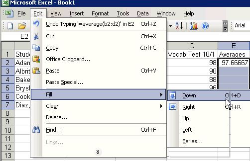
• Tada! Now, all students' grades are averaged.
• Save your work.

Next: Formatting and printing the grade book.